Latest Release

Fixed bugs in the legend of the CV summary plot and in colouring the observations in the PLSS (t_i,t_j) scatterplots

The release 2024/04/01 of the function Bsplines presents a new input cex.labpar allowing to magnify x and y axis labels

in the plot of the perturbed identity spline. The left plot below is obtained as the output of the Bsplines R function and

the two plots are now published in "Statistical Methods & Applications"

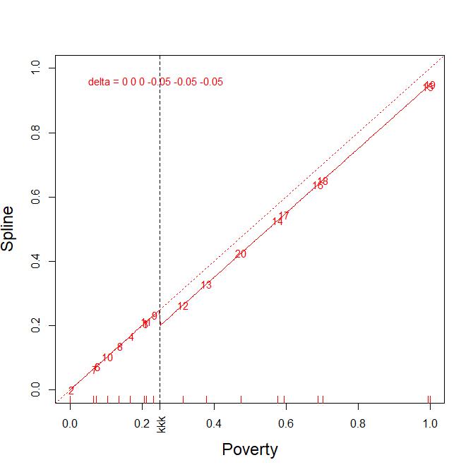
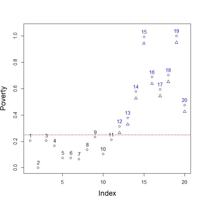
Italian regions Poverty 1 Italian regions Poverty 2

Poverty in the 20 regions of Italy. Left plot, the identity spline (red dotted line) of degree 2, 1 knot of multiplicity 3

at the mean Poverty value 0.25. The delta values locally perturb by -0.05 the nodal coefficients of the identity spline

only on the nine regions above the threshold 0.25. Right plot in blue, the nine regions and their delta scenario -0.05.

Release 23.00
The function Bsplines replaces the old one Bspline. To have a look at the changes see the latest version of the report
"Short guide to the function Bsplines" whose aim is to get acquainted with the B-splines basis functions in both statistical and CAID domains.
This new release allows to manage online some variations around the spline identity based on nodal weights. Nodal values are also shown in
the context of approximation splines by the Bsplines function.
Moreover, barplots are now presenting horizontal bars with horizontal names in the left margin.
Release 20.92
Some improvements in displaying the CV and GCV plots of the campaign of experimenting different number of observations out at a time for
the Cross-Validation (CV) and different alpha parameters in the Generalysed Cross-Validation (GCV).

Release 20.91
The centroïds of the groups in the discriminant component (ti,tj) plots are correctly displayed when (ti,tj) not (1,2).
Some little bugs displaying the threshold of acceptability in the PRESS plots have been removed.
The title of the MVcut plot (see below) is now more conveniently displayed.

Release 20.90
Two new auxiliary R-functions:   Hotelling and HotellingEllipse

Description:
Allows to detect T² ouliers using the PCA or the PLS components and display T² Hotelling ellipses on the same (ti, tj) scatterplot.
Hotelling: to detect outlying observations on the component variables ii and jj (default to 1 and 2) at the Fisher-Snedecor level (FSthreshold defaults to 0.95).
   Hotelling displays the corresponding T² ellipse only if FStrhesold=0.95 thus giving the initial plot.
HotellingEllipse: When FSthreshold is different from 0.95 one have to use Hotelling and then HotellingEllipse to see the ellipse and the coloured outliers.

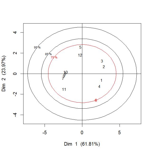
Example ; PCA on 'cornell' data (see Tenenhaus's book on pages 86-87   or the lecture notes, page 199)
.
                                    cornellPCA=acpxqd(cornell,bgpar="white")
                               Hotelling(cornellPCA$C, axislabel=list("Dim 1 (61.81%)","Dim 2 (23.97%)") )
                          HOTcornell85 = Hotelling(cornellPCA$C, FSthreshold=0.85)
                          HotellingEllipse(HOTcornell85, colpar="black")
                         HOTcornell75 = Hotelling(cornellPCA$C, FSthreshold=0.75)
                         [1] "Outliers with components 1 and 2 ,T²=75% :"
                        [1] "6"
                          HotellingEllipse(HOTcornell75, colpar="red")

Release 20.80
1) Numerical outputs in the PLS iterations are differently displayed in the one response case. The adjusted R² is now computed.

   > PLSL(cornell[,1:7],cornell[,8,drop=F], cexpar=0.8,bgpar="white")
            - Linear PLS -
   Total Variance of X = 7
   Variance of y = 1 , y0 = y

   Dimension 1

cov(t1,y0)= 1.916 r(t1,y0)= 0.961 stdev(t1)= 1.994 stdev(y0)= 1

              y    % of VAR
   R2 part. 0.924    92.359
..................
   adjusted R2 for y with dim. 1 and 7 predictors : R2_adjust= 0.791
. .................
   % of VAR X accounted for by the current comp. = 57.361

2) PRESS plots can eventually show the threshold of acceptability for the dimension of the model.

The rule for the dimension k, being (in the 1 response case):

PRESS(k) > 1 ==> model not better than yhat(k) = mean(y)= 0, PRESS(k) = 1 = var(y)

Release 20.69
1) A new MVcut R-function to code continuous vaviables into categorical by choosing graphically the breaks points that default to quantiles.

     Heavylevel=MVcut(juice[,11,drop=F],graph=T)
     Heavy :
     nunber of levels : 3

Change or not that number ? (y/n)1:

2) The item "Remove/Add variables" no more available in the MAPLSS menu.